shinyDSP internal data processing pipeline explained

Seung J. Kim

Interstitial Lung Disease Lab, London Health Sciences Center
skim823@uwo.ca

Marco Mura

Interstitial Lung Disease Lab, London Health Sciences CenterDivision of Respirology, Department of Medicine, Western University
marco.mura@respirology.site.co

12 June 2025

Source: vignettes/shinyDSP_secondary.Rmd

shinyDSP_secondary.Rmd

Introduction

The purpose of this vignette is to look under the hood and explain what a few underlying functions do to make this app work.

Data import

The human kidney data from Nanostring is loaded from ExperimentHub(). Two files are required: a count matrix and matching annotation file. Let’s read those files.

library(standR)
library(SummarizedExperiment)
library(ExperimentHub)
library(readr)
library(dplyr)
library(stats)

eh <- ExperimentHub()
AnnotationHub::query(eh, "standR")

## ExperimentHub with 3 records
## # snapshotDate(): 2025-04-12
## # $dataprovider: Nanostring
## # $species: NA
## # $rdataclass: data.frame
## # additional mcols(): taxonomyid, genome, description,
## #   coordinate_1_based, maintainer, rdatadateadded, preparerclass, tags,
## #   rdatapath, sourceurl, sourcetype 
## # retrieve records with, e.g., 'object[["EH7364"]]' 
## 
##            title                   
##   EH7364 | GeomxDKDdata_count      
##   EH7365 | GeomxDKDdata_sampleAnno 
##   EH7366 | GeomxDKDdata_featureAnno

countFilePath <- eh[["EH7364"]]
sampleAnnoFilePath <- eh[["EH7365"]]

countFile <- readr::read_delim(unname(countFilePath), na = character())
sampleAnnoFile <- readr::read_delim(unname(sampleAnnoFilePath), na = character())

Time for this code chunk to run: 2.53 seconds

Variable(s) selection

A key step in analysis is to select a biological group(s) of interest. Let’s inspect sampleAnnoFile.

colnames(sampleAnnoFile)

##  [1] "SlideName"            "ScanName"             "ROILabel"            
##  [4] "SegmentLabel"         "SegmentDisplayName"   "Sample_ID"           
##  [7] "AOISurfaceArea"       "AOINucleiCount"       "ROICoordinateX"      
## [10] "ROICoordinateY"       "RawReads"             "TrimmedReads"        
## [13] "StitchedReads"        "AlignedReads"         "DeduplicatedReads"   
## [16] "SequencingSaturation" "UMIQ30"               "RTSQ30"              
## [19] "disease_status"       "pathology"            "region"              
## [22] "LOQ"                  "NormalizationFactor"  "RoiReportX"          
## [25] "RoiReportY"

sampleAnnoFile$disease_status %>% unique()

## [1] "DKD"    "normal"

sampleAnnoFile$region %>% unique()

## [1] "glomerulus" "tubule"

“disease_status” and “region” look like interesting variables. For example, we might be interested in comparing “normal_glomerulus” to “DKD_glomerulus”. The app can create a new sampleAnnoFile where two or more variables of interest can be combined into one grouped variable (under “Variable(s) of interest” in the main side bar).

new_sampleAnnoFile <- sampleAnnoFile %>%
    tidyr::unite(
        "disease_region", # newly created grouped variable
        c("disease_status","region"), # variables to combine
        sep = "_"
    )

new_sampleAnnoFile$disease_region %>% unique()

## [1] "DKD_glomerulus"    "DKD_tubule"        "normal_tubule"    
## [4] "normal_glomerulus"

Time for this code chunk to run: 0.01 seconds

Finally a spatial experiment object can be created.

spe <- standR::readGeoMx(as.data.frame(countFile),
                         as.data.frame(new_sampleAnnoFile))

Time for this code chunk to run: 0.31 seconds

Selecting groups to analyze

We merged “disease_status” and “region” to create a new group called, “disease_region”. The app allows users to pick any subset of groups of interest. In this example, the four possible groups are “DKD_glomerulus”, “DKD_tubule”,“normal_tubule”, and “normal_glomerulus”. The following script can subset spe to keep certain groups.

selectedTypes <- c("DKD_glomerulus", "DKD_tubule", "normal_tubule", "normal_glomerulus")
toKeep <- colData(spe) %>%
    tibble::as_tibble() %>%
    pull(disease_region)

spe <- spe[, grepl(paste(selectedTypes, collapse = "|"), toKeep)]

Time for this code chunk to run: 0.03 seconds

Applying QC filters

Regions of interest(ROIs) can be filtered out based on any quantitative variable in colData(spe) (same as colnames(new_sampleAnnoFile)). These options can be found under the “QC” nav panel’s side bar. Let’s say I want to keep ROIs whose “SequencingSaturation” is at least 85.

filter <- lapply("SequencingSaturation", function(column) {
    cutoff_value <- 85
    if(!is.na(cutoff_value)) {
        return(colData(spe)[[column]] > cutoff_value)
    } else {
        return(NULL)
    }
})

filtered_spe <- spe[,unlist(filter)]

colData(spe) %>% dim()

## [1] 231  24

colData(filtered_spe) %>% dim()

## [1] 217  24

Time for this code chunk to run: 0.02 seconds

We can see that 14 ROIs have been filtered out.

PCA

Two PCA plots (colour-coded by biological groups or batch) for three normalization schemes are automatically created in the “PCA” nav panel. Let’s take Q3 and RUV4 normalization as an example.

speQ3 <- standR::geomxNorm(filtered_spe, method = "upperquartile")
speQ3 <- scater::runPCA(filtered_spe)

speQ3_compute <- SingleCellExperiment::reducedDim(speQ3, "PCA")

Time for this code chunk to run: 0.63 seconds

speRuv_NCGs <- standR::findNCGs(filtered_spe,
        batch_name = "SlideName",
        top_n = 200)


speRuvBatchCorrection <- standR::geomxBatchCorrection(speRuv_NCGs,
            factors = "disease_region",
            NCGs = S4Vectors::metadata(speRuv_NCGs)$NCGs, k = 2
        )

speRuv <- scater::runPCA(speRuvBatchCorrection)

speRuv_compute <- SingleCellExperiment::reducedDim(speRuv, "PCA")

Time for this code chunk to run: 3.04 seconds

Then, .PCAFunction() is called to generate the plot. We can see that biological replicates group better with RUV4 (top) compared to Q3 (bottom).

.PCAFunction(speRuv, speRuv_compute, "disease_region", selectedTypes, c(21,22,23,24), c("blue","dodgerblue1","black","grey75"))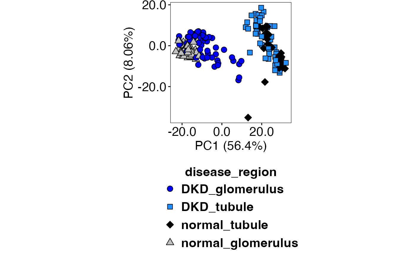

.PCAFunction(speQ3, speQ3_compute, "disease_region", selectedTypes, c(21,22,23,24), c("blue","dodgerblue1","black","grey75"))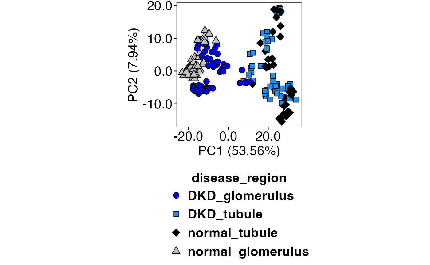

Time for this code chunk to run: 0.26 seconds

Design matrix

Let’s proceed with RUV4 normalization. A design matrix is created next.

design <- model.matrix(~0+disease_region+ruv_W1+ruv_W2, data = colData(speRuv))

# Clean up column name
colnames(design) <- gsub("disease_region", "", colnames(design))

Time for this code chunk to run: 0.01 seconds

If confounding variables are chosen in the main side bar, those would be added to model.matrix as ~0 + disease_region + confounder1 + confounder2).

Creating a DGEList

edgeR is used to convert SpatialExperiment into DGEList, filter and estimate dispersion.

library(edgeR)
dge <- SE2DGEList(speRuv)
keep <- filterByExpr(dge, design)

dge <- dge[keep, , keep.lib.sizes = FALSE]

dge <- estimateDisp(dge, design = design, robust = TRUE)

Time for this code chunk to run: 11.84 seconds

Comparison between all biological groups

Recall our “selectedTypes” from above: “DKD_glomerulus”, “DKD_tubule”, “normal_tubule”, “normal_glomerulus”.

The following code creates all pairwise comparisons between them.

# In case there are spaces
selectedTypes_underscore <- gsub(" ", "_", selectedTypes)

comparisons <- list()

comparisons <- lapply(
    seq_len(choose(length(selectedTypes_underscore), 2)),
    function(i) {
        noquote(
            paste0(
                utils::combn(selectedTypes_underscore, 2,
                    simplify = FALSE
                )[[i]][1],
                "-",
                utils::combn(selectedTypes_underscore, 2,
                    simplify = FALSE
                )[[i]][2]
            )
        )
    }
)

con <- makeContrasts(
    # Must use as.character()
    contrasts = as.character(unlist(comparisons)),
    levels = colnames(design)
)

colnames(con) <- sub("-", "_vs_", colnames(con))

con

##                    Contrasts
## Levels              DKD_glomerulus_vs_DKD_tubule
##   DKD_glomerulus                               1
##   DKD_tubule                                  -1
##   normal_glomerulus                            0
##   normal_tubule                                0
##   ruv_W1                                       0
##   ruv_W2                                       0
##                    Contrasts
## Levels              DKD_glomerulus_vs_normal_tubule
##   DKD_glomerulus                                  1
##   DKD_tubule                                      0
##   normal_glomerulus                               0
##   normal_tubule                                  -1
##   ruv_W1                                          0
##   ruv_W2                                          0
##                    Contrasts
## Levels              DKD_glomerulus_vs_normal_glomerulus
##   DKD_glomerulus                                      1
##   DKD_tubule                                          0
##   normal_glomerulus                                  -1
##   normal_tubule                                       0
##   ruv_W1                                              0
##   ruv_W2                                              0
##                    Contrasts
## Levels              DKD_tubule_vs_normal_tubule DKD_tubule_vs_normal_glomerulus
##   DKD_glomerulus                              0                               0
##   DKD_tubule                                  1                               1
##   normal_glomerulus                           0                              -1
##   normal_tubule                              -1                               0
##   ruv_W1                                      0                               0
##   ruv_W2                                      0                               0
##                    Contrasts
## Levels              normal_tubule_vs_normal_glomerulus
##   DKD_glomerulus                                     0
##   DKD_tubule                                         0
##   normal_glomerulus                                 -1
##   normal_tubule                                      1
##   ruv_W1                                             0
##   ruv_W2                                             0

Time for this code chunk to run: 0.01 seconds

Fitting a linear regression model with `limma`

The app uses duplicateCorrelation() “[s]ince we need to make comparisons both within and between subjects, it is necessary to treat Patient as a random effect” limma user’s guide (Ritchie et al. 2015). limma-voom method is used as standR package recommends (Liu et al. 2024).

library(limma)
block_by <- colData(speRuv)[["SlideName"]]

v <- voom(dge, design)
corfit <- duplicateCorrelation(v, design,
    block = block_by
)

v2 <- voom(dge, design,
    block = block_by,
    correlation = corfit$consensus
)

corfit2 <- duplicateCorrelation(v, design,
    block = block_by
)

fit <- lmFit(v, design,
    block = block_by,
    correlation = corfit2$consensus
)

fit_contrast <- contrasts.fit(fit,
    contrasts = con
)

efit <- eBayes(fit_contrast, robust = TRUE)

Time for this code chunk to run: 48.03 seconds

Tables of top differentially expressed genes

For each contrast (a column in con), the app creates a table of top differentially expressed genes sorted by their adjusted P value.

# Keep track of how many comparisons there are
numeric_vector <- seq_len(ncol(con))
new_list <- as.list(numeric_vector)

# This adds n+1th index to new_list where n = ncol(con)
# This index contains seq_len(ncol(con)) 
# ex. new_list[[7]] = 1 2 3 4 5 6
# This coefficient allows ANOVA-like comparison in toptable()
if (length(selectedTypes) > 2) {
    new_list[[length(new_list) + 1]] <- numeric_vector
}

topTabDF <- lapply(new_list, function(i) {
    limma::topTable(efit,
        coef = i, number = Inf, p.value = 0.05,
        adjust.method = "BH", lfc = 1
    ) %>%
        tibble::rownames_to_column(var = "Gene")
})

# Adds names to topTabDF
if (length(selectedTypes) > 2) {
    names(topTabDF) <- c(
        colnames(con),
        colnames(con) %>% stringr::str_split(., "_vs_") %>%
            unlist() %>% unique() %>% paste(., collapse = "_vs_")
    )
} else {
    names(topTabDF) <- colnames(con)
}

Time for this code chunk to run: 0.03 seconds

topTabDF is now a list of tables where the list index corresponds to that of columns in con.

colnames(con)

## [1] "DKD_glomerulus_vs_DKD_tubule"        "DKD_glomerulus_vs_normal_tubule"    
## [3] "DKD_glomerulus_vs_normal_glomerulus" "DKD_tubule_vs_normal_tubule"        
## [5] "DKD_tubule_vs_normal_glomerulus"     "normal_tubule_vs_normal_glomerulus"

head(topTabDF[[1]])

##      Gene Type mean_zscore mean_expr    logFC  AveExpr        t      P.Value
## 1 SRGAP2B gene    5.392825  8.094697 2.591325 8.064988 30.74096 1.974029e-80
## 2   PODXL gene   11.146967  8.563414 4.502203 8.518927 30.81248 4.080221e-80
## 3    FGF1 gene    8.865378  7.692389 3.539804 7.632976 30.30632 7.097517e-79
## 4   CLIC5 gene    9.624410  7.925377 3.780739 7.869413 29.14067 5.750702e-76
## 5    PLAT gene    8.262970  8.297025 3.965194 8.256626 29.08766 7.827953e-76
## 6  SPOCK1 gene    5.899207  7.119840 2.745986 7.061100 28.75805 6.656020e-76
##      adj.P.Val        B
## 1 3.628068e-76 172.6863
## 2 3.749520e-76 171.7997
## 3 4.348175e-75 168.8320
## 4 2.397832e-72 162.3045
## 5 2.397832e-72 162.1593
## 6 2.397832e-72 162.1138

These tables are then shown to the user in the “Tables” nav panel.

Volcano plot and heatmap

No further serious data processing is performed at this point. The numbers in topTabDF is now parsed to create volcano plots and heatmaps in their respective nav panels.

volcanoDF <- lapply(seq_len(ncol(con)), function(i) {
                limma::topTable(efit, coef = i, number = Inf) %>%
                    tibble::rownames_to_column(var = "Target.name") %>%
                    dplyr::select("Target.name", "logFC", "adj.P.Val") %>%
                    dplyr::mutate(de = ifelse(logFC >= 1 &
                        adj.P.Val < 0.05, "UP",
                    ifelse(logFC <= -(1) &
                        adj.P.Val < 0.05, "DN",
                    "NO"
                    )
                    )) %>%
                    dplyr::mutate(
                        logFC_threshold = stats::quantile(abs(logFC), 0.99,
                            na.rm = TRUE
                        ),
                        pval_threshold = stats::quantile(adj.P.Val, 0.01,
                            na.rm = TRUE
                        ),
                        deLab = ifelse(abs(logFC) > logFC_threshold &
                            adj.P.Val < pval_threshold &
                            abs(logFC) >= 0.05 &
                            adj.P.Val < 0.05, Target.name, NA)
                    )
            })

plots <- lapply(seq_along(volcanoDF), function(i) {
    .volcanoFunction(
        volcanoDF[[i]], 12, 5,
        colnames(con)[i],
        1, 0.05,
        "Blue", "Grey", "Red"
    ) +
        ggplot2::xlim(
            -2,
            2
        ) +
        ggplot2::ylim(
            0, 20
        )
})

plots[1]

## [[1]]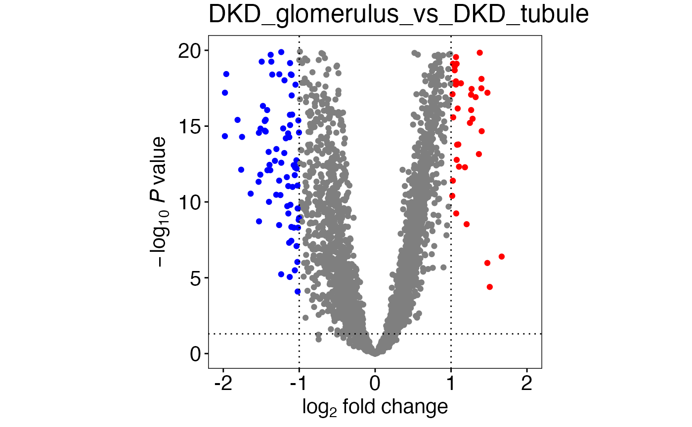

Time for this code chunk to run: 0.44 seconds

In contrast to Volcano plots, only the top N genes are shown in a heatmap. Setup is a bit more involved.

lcpmSubScaleTopGenes <- lapply(names(topTabDF), function(name) {
            columns <- stringr::str_split_1(name, "_vs_") %>%
                lapply(function(.) {
                    which(SummarizedExperiment::colData(speRuv) %>%
                        tibble::as_tibble() %>%
                        dplyr::pull(disease_region) == .)
                }) %>%
                unlist()

            table <- SummarizedExperiment::assay(speRuv, 2)[
                topTabDF[[name]] %>%
                    dplyr::slice_head(n = 50) %>%
                    dplyr::select(Gene) %>%
                    unlist() %>%
                    unname(),
                columns
            ] %>%
                data.frame() %>%
                t() %>%
                scale() %>%
                t()

            return(table)
        })

        names(lcpmSubScaleTopGenes) <- names(topTabDF)
        
columnSplit <- lapply(names(topTabDF), function(name) {
    columnSplit <- stringr::str_split_1(name, "_vs_") %>%
        lapply(function(.){
            which(
                SummarizedExperiment::colData(speRuv) %>%
                    tibble::as_tibble() %>% dplyr::select(disease_region) == .
            )
        } ) %>%
        as.vector() %>%
        summary() %>%
        .[, "Length"]
})

names(columnSplit) <- names(lcpmSubScaleTopGenes)

Time for this code chunk to run: 0.22 seconds

colFunc <- circlize::colorRamp2(
            c(
                -3, 0,
                3
            ),
            hcl_palette = "Inferno"
        )

heatmap <- lapply(names(lcpmSubScaleTopGenes), function(name) {
    ComplexHeatmap::Heatmap(lcpmSubScaleTopGenes[[name]],
        cluster_columns = FALSE, col = colFunc,
        heatmap_legend_param = list(
            border = "black",
            title = "Z score",
            title_gp = grid::gpar(
                fontsize = 12,
                fontface = "plain",
                fontfamily = "sans"
            ),
            labels_gp = grid::gpar(
                fontsize = 12,
                fontface = "plain",
                fontfamily = "sans"
            ),
            legend_height = grid::unit(
                3 * as.numeric(30),
                units = "mm"
            )
        ),
        top_annotation = ComplexHeatmap::HeatmapAnnotation(
            foo = ComplexHeatmap::anno_block(
                gp = grid::gpar(lty = 0, fill = "transparent"),
                labels = columnSplit[[name]] %>% names(),
                labels_gp = grid::gpar(
                    col = "black", fontsize = 14,
                    fontfamily = "sans",
                    fontface = "bold"
                ),
                labels_rot = 0, labels_just = "center",
                labels_offset = grid::unit(4.5, "mm")
            )
        ),
        border_gp = grid::gpar(col = "black", lwd = 0.2),
        row_names_gp = grid::gpar(
            fontfamily = "sans",
            fontface = "italic",
            fontsize = 10
        ),
        show_column_names = FALSE,
        column_title = NULL,
        column_split = rep(
            LETTERS[seq_len(columnSplit[[name]] %>% length())],
            columnSplit[[name]] %>% unname() %>% as.numeric()
        )

    )
})

names(heatmap) <- names(lcpmSubScaleTopGenes)

heatmap[[1]]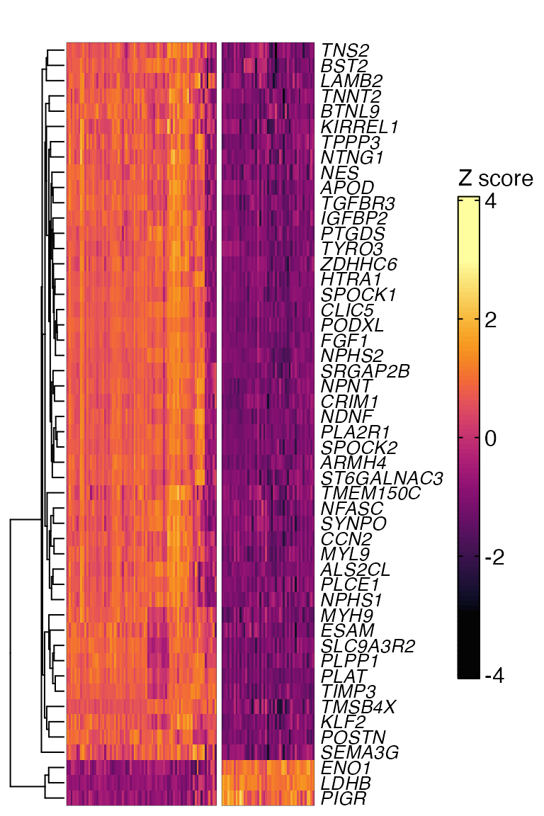

Time for this code chunk to run: 0.65 seconds

Liu, Ning, Dharmesh D Bhuva, Ahmed Mohamed, Micah Bokelund, Arutha Kulasinghe, Chin Wee Tan, and Melissa J Davis. 2024. “standR: Spatial Transcriptomic Analysis for GeoMx DSP Data.” Nucleic Acids Research 52 (1): e2–2. https://doi.org/10.1093/nar/gkad1026.

Ritchie, Matthew E., Belinda Phipson, Di Wu, Yifang Hu, Charity W. Law, Wei Shi, and Gordon K. Smyth. 2015. “Limma Powers Differential Expression Analyses for RNA-Sequencing and Microarray Studies.” Nucleic Acids Research 43 (7): e47–47. https://doi.org/10.1093/nar/gkv007.

shinyDSP internal data processing pipeline explained

Seung J. Kim

Marco Mura

12 June 2025

Introduction

Data import

Variable(s) selection

Selecting groups to analyze

Applying QC filters

PCA

Design matrix

Creating a DGEList

Comparison between all biological groups

Fitting a linear regression model with limma

Tables of top differentially expressed genes

Volcano plot and heatmap

Fitting a linear regression model with `limma`